
In the previous tutorial, we talked about Linear Regression, and we used it to predict house prices using size of the house as a feature. Linear Regression is great if we are trying to predict real valued outcomes like house prices, but not so great if we want to predict whether something belongs in a certain category or not. In Linear Classification, our goal is to fit a line that separates our data into two classes, and use that line to predict the class of unseen data.

Suppose your boss assigns you as a hiring manager and tells you to take on his job of hiring software engineers. The only problem is, he doesn't tell you what to look for in the applicants. He hands you a list of past applicants with three fields: GPA, IQ and whether they were hired or not. being the lazy engineer you've always been, you decide to write a script that uses a linear classifier to automate the task using the data given by your boss.
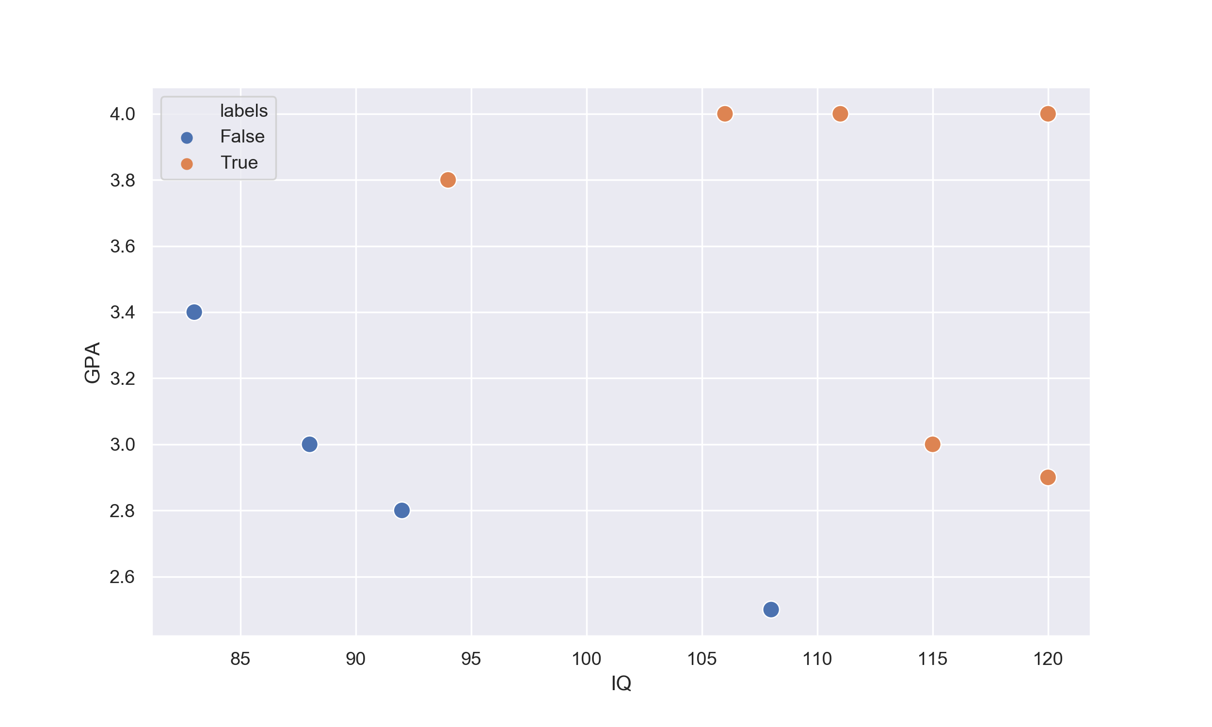
$$ \begin{array}{c|c|c|c} n & \text{IQ} & \text{GPA} & \text{Hired} \\ \hline 1 & 88 & 3.0 & No\\ 2 & 120 & 2.9 & Yes\\ 3 & 111 & 4.0 & Yes\\ 4 & 83 & 3.4 & No\\ 5 & 94 & 3.8 & Yes\\ 6 & 106 & 4.0 & Yes\\ 7 & 108 & 2.5 & No\\ 8 & 92 & 2.8 & No\\ 9 & 108 & 3.0 & Yes\\ 10 & 92 & 4.0 & Yes\\ \end{array} $$If we plot the data on a scatter plot, we will get a graph like this:

# Initializing the data in Python
IQ = [88, 120, 111, 83, 94, 106, 108, 92, 115, 120]
GPA = [3.0, 2.9, 4.0, 3.4, 3.8, 4.0, 2.5, 2.8, 3.0, 4.0]
labels = [0.0, 1.0, 1.0, 0.0, 1.0, 1.0, 0.0, 0.0, 1.0, 1.0]
The goal of a linear classifier is to learn a line (in the case of 2D), or a hyperplane (in the case of 3D+), that separates the data. Because we are dealing with two features, namely GPA and IQ, our model is going to be a 2D line in the form:
$$f(x_{1},x_{2}) = \theta_{0}x_{0} + \theta_{1}x_{1} + \theta_{2}x_{2},$$where $\theta_{1}$ and $\theta_{2}$ are the two coefficients of the line, $x_{1}$ and $x_{2}$ are our two features we have for each applicant. Just like in the previous tutorial, we will be initializing the coefficients to small values between -1 and 1:
$$ f(x_{1},x_{2}) = 1.0x_{0} + 1.0x_{1} + 1.0x_{2} $$We will be using numpy arrays for this tutorial as it is much simpler to do vector dot products than to manually sum the multiplications of the coefficients and features. Now our equation should look like this:
$$ f(x_{1}, x_{2}) = W \cdot X =\begin{bmatrix} \theta_{0} \\ \theta_{1} \\ \theta_{2} \end{bmatrix} \cdot \begin{bmatrix} x_{0} & x_{1} & x_{2} \end{bmatrix}$$Before we train our function which we will be referring to as the model from this point on - we need to make the values of the features smaller by normalizing them. If you don't know about normalization, check out my previous tutorial.
# Initializing the function coefficients
coefficient = np.array([1.0, 1.0, 1.0])

# Creating the feature matrix
examples = np.ones((3,10))
examples[1] = normalize(IQ)
examples[2] = normalize(GPA)
There are many well known linear classifier algorithms such as Winnow, but I will be going over the Perceptron algorithm as it is the most popular.
So far, everything has been the same as the linear classifier. We have a list of points on a 2D plot, and we initialized a 2D linear function, but this is where things start to change. We will now choose something called a $threshold$, which will be used to classify the output of the function for each applicant in the following way:
$$ f(x_{1},x_{2}) = \begin{cases} 0 & f(x_{1},x_{2}) < threshold \\ 1 & f(x_{1},x_{2}) \ge threshold \end{cases} $$where 0 is not hired and 1 is hired. In our perceptron example, we will be using a threshold of 0, but feel free to see how different thresholds affect the learning. So let's now see how much our model with arbitrary coefficients performs. The output of the first example is
$$ f(x_{1}, x_{2}) = W \cdot X =\begin{bmatrix} 1.0 \\ 1.0 \\ 1.0 \end{bmatrix} \cdot \begin{bmatrix} 1.0 & -0.42 & -0.23 \end{bmatrix} = 0.35 $$Since out threshold is 0, the output is hired - which isn't what we want. So let's now update the coefficients using the perceptron algorithm. The algorithm is as follows:
$$ \theta_{j} := \theta_{j} + (target-f(x,y))x_{j}, $$where $\theta_{j}$ is the $j_{th}$ coefficient, $target$ is the desired outcome, $f(x_{1},x_{2})$ is the output of our function, and $x_{j}$ is the $j_{th}$ feature value that corresponds to the coefficient.
def test(examples):
    error = 0
    global coefficient
    for example, label in zip(examples.T, labels):
        output = coefficient.dot(example.T)
        if output > 0:
            output = 1
        else:
            output = 0
        error += label - output
    return error/len(examples)

def train(examples, epochs=25):
    global coefficient
    for i in range(1, epochs + 1):
        for example, label in zip(examples.T, labels):
            output = coefficient.dot(example.T)
            if output > 0:
                output = 1
            else:
                output = 0
            error = label - output
            coefficient += 0.01*error*example
		e = test(examples)
		print("Error at {} epochs: {}".format(i,e))
Now that's we've learnt everything we need to implement the perceptron linear classifier, let's test it out!
train(examples)
Error at 5 epochs:	-1.3333333333333333
Error at 10 epochs:	-0.6666666666666666
Error at 15 epochs:	-0.3333333333333333
Error at 20 epochs:	0.0
Error at 25 epochs:	0.0
We can see here that after 20 epochs, the algorithm managed to learn the data!
Congratulations, we have successfully implemented a Linear Classifier!