
You might've come across the term 'line of best fit' at school if you took an introductory statistics course. Simply put, it is line on a scatter plot that goes through the middle of all data points. In the case of a two dimensional plot, this line will be $y=mx+b$.
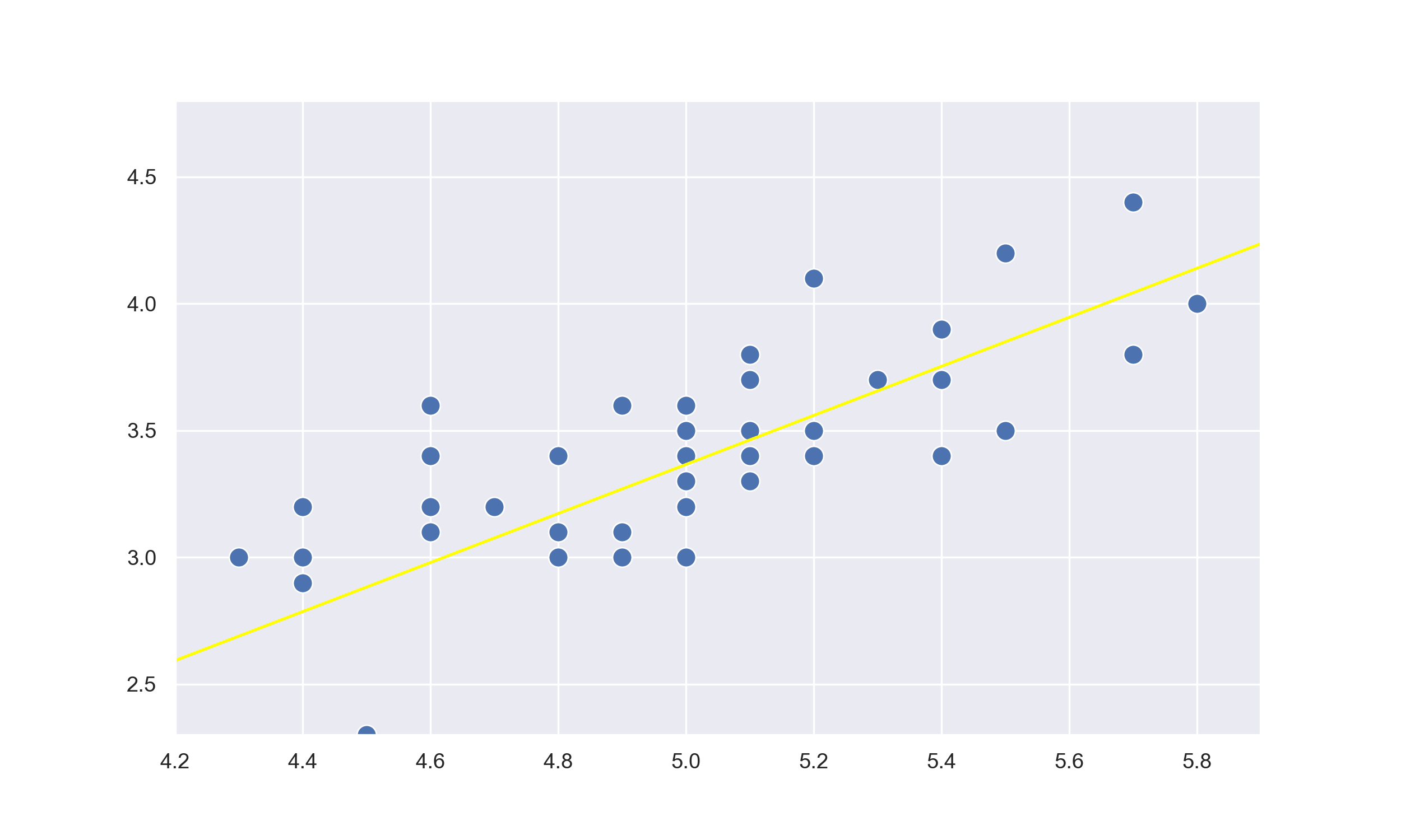
The idea behind linear regression in machine learning is to find the 'line of best fit' using mathematics and the processing power of modern day computers to calculate the line that best represents the data.
Suppose you are trying to sell your house and you are given a list of other houses on sale. A typical posting may contain attributes such as size in squared meters, number of bedrooms, and number of carparks, but you can't seem to find a house with similar attributes. The question you might want to ask is, "How can I use the postings list to infer an appropriate price for my house?" Luckily, this problem can be solved used linear regression.
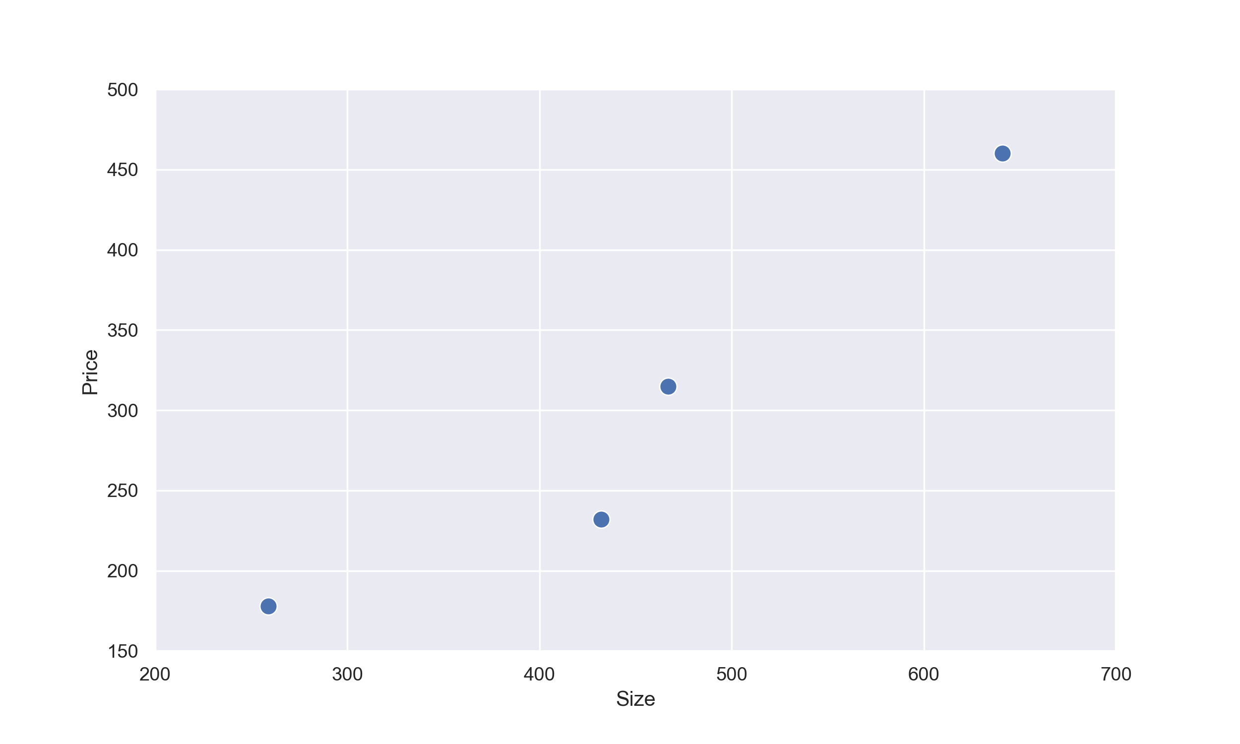
For sake of argument, let's only use the size of the houses to infer the price of your house. Below is a list of house sizes and their corresponding house prices around your area.
$$ \begin{array}{c|c|c} n & \text{Size ($m^{2}$)} & \text{Price} \\ \hline 1 & 641 & 460 \\ 2 & 432 & 232 \\ 3 & 467 & 315 \\ 4 & 259 & 178 \end{array} $$If we plot the data on a scatter plot, we will get a graph like this:
# Initializing the data in Python
size = [641.0, 432.0, 467.0, 259.0]
price = [460.0, 232.0, 315.0, 178.0]
So now the question is, "How can we perform linear regression on the data to fit a line?". In order to perform linear regression, we first need to start with a random equation of a line in the form of:
$$ f(x) = \theta_{0}x_{0} + \theta_{1}x_{1}, $$where $\theta_{0}$ and $\theta_{1}$ are the two coefficients of the line, namely the y intercept and the slope, $x_{0}$ is always 1 and $x_{1}$ is the size of the house. Furthermore, the coefficients should be randomly chosen between -0.5 and 0.5. There is a good explanation as to why it should be between this range, but as it is beyond the scope of this tutorial, let's just say it's good practice.
The following is an arbitrarily created equation we will be using for the rest of this tutorial:
$$ f(x) = -0.25x_{0} + 0.25x_{1} $$
# Initializing the function coefficients
coefficient = [-0.25, 0.25]
The general approach in linear regression is to start with a randomized equation of a line, and slowly 'tweak' the coefficients of the equation to get as close as possible to the correct position. Before we can even attempt to tweak the coefficients, we need to figure out how off our randomized line is. We can do this by calculating how far each point is from the line, a.k.a. calculating the mean squared error (MSE). The formula for MSE is the following:
$$ J(\theta_{0},\theta_{1}) = {{1 \over n} \sum^{n}_{i=1}{(f(x)-y)^{2}}}.$$Here $f(x)$ refers to the equation of the line we created earlier, y refers to the actual value we are trying to predict, and n is the number of data points we have. If we replace these variables with values we are concerned with for predicting house prices, we will get the following:
$$ \begin{align}J(\theta_{0},\theta_{1}) &= \small \frac{(160 - 460)^{2} + (107.75 - 232)^{2} + (116.5 - 315)^{2} + (64.5 - 178)^{2}}{4} \\ &= 39430.64. \end{align}$$
According to MSE, we have an error of 39430.64, which is a pretty large error. This is because the the size of the houses are quite large relative to the coefficients of the function and we must normalize them so we start with a smaller error and it does not take forever to find the line of best fit. The method we are going to use to normalize the size of the houses is
$$ x' = \frac{x-\bar{x}}{max(x)-min(x)},$$where $x$ is the original value of the size, $\bar{x}$, $max$ and $min$ are the mean, maximum and minimum of the size of houses respectively. Keep in mind that as the points are not lined up properly, it is impossible for us to get an error of zero. This turns out to be the case in most scenarios when we are dealing with real world problems.
# Normalize values
def normalize(x):
    mean = sum(x)/float(len(x))
    minimum = min(x)
    maximum = max(x)
    return [(i-mean)/(maximum-minimum) for i in x]
Now that we have calculated the error, we want to decrease the error as much as we can using derivatives. If you are unfamiliar with derivatives, I strongly encourage you to watch a great series on derivates here.
So how can we minimize the error produced by the MSE formula? One way to approach this problem is to calculate the derivative of the MSE function - which we will call the $error$ $function$ from this point on, using the chain rule and equate it to zero. I have already found the derivative for you below:
$$ \begin{align} \frac{d}{d \theta_{j}}(J(\theta_{0},\theta_{1}) &= \frac{d}{d \theta_{j}}\left({1 \over n} \sum^{n}_{i=1}{(f(x)-y)^{2}}\right) \\ &= {2 \over n} \sum^{n}_{i=1}{(f(x)-y)x_{j}}. \end{align} $$
# Compute the MSE and its derivative
def mse(x, y, deriv=False):
    error = []
    for data, target in zip(x,y):
	pred = coefficient[0] + coefficient[1] * data
        if deriv == True:
            error.append(2 * (pred - target) / len(x))
        else:
            error.append(((pred - target) ** 2) / len(x))
    return error
At this point, we have learnt all the tools we need to fit a line of best fit to our data. Our next step is use a method called Gradient Descent which uses the gradient of the error function to move our error to the minimum of the error function. The formula for gradient descent is the following:
$$ \theta_{j} := \theta_{j} - a \frac{d}{d\theta_{j}}J(\theta_{0},\theta_{1}).$$where $\theta_{j}$ is the $j_{th}$ coefficient of our equation, $a$ is the learning rate which is a constant that should be smaller than 1, and $\frac{d}{d\theta_{j}}(J(\theta_{0},\theta_{1}))$ is the derivative of the error function with respect to the $j_{th}$ coefficient. The function may look daunting at first, but all it is doing is slightly changing the coefficients of our current line equation in the opposite direction of gradient which is controlled by learning rate. The learning rate is very important here because it determines the size of the step you take in the direction. This means if the learning rate is too large, the algorithm may overshoot the minimum and attempt to go backwards, but will keep overshooting as the steps are too large. To get a better understanding of how the learning rate affects the algorithm, I strongly encourage you to experiment with different rates between 1 and 0.00001.
Before we move on, the concept of $epochs$ must be discussed. The update method that we have arrived at only minimizes the error by a very small amount. In order for the error to be minimized as much as much possible, we must repeat the update process several times. In machine learning, there is a special term called $epochs$, which refers to the number of times an update is performed. For this example, we will choose 1000, but feel free to experiment with smaller and larger values to see how it affects our line.
# Calculate the error of our line
def test(x, y):
    error = sum(mse(x, y))
    return error

# Perform gradient descent
def gradient_descent(x, y, epoch=1000):
    lr = 0.01 # Learning rate
    for i in range(epoch):
        error_theta_0 = mse(x, y, deriv=True)
        error_theta_1 = [error_theta_0[i] * val for val in x]
        coefficient[0] -= lr*sum(error_theta_0)
        coefficient[1] -= lr*sum(error_theta_1)
        if i % 100 == 0:
	    error = test(x,y)
	    print("Error at {} epochs: {}".format(i, error))
Now that we've learnt and coded everything we need to find the line of best fit, we can run the code to test how we have done!
size_norm = normalize(size)
gradient_descent(size_norm, price)
If you got the following output, then we've successfully implemented linear regression!
Error at 0 epochs: 95679.70737917697
Error at 100 epochs: 8637.12391268404
Error at 200 epochs: 4705.53249958228
Error at 300 epochs: 3187.3153746545486
Error at 400 epochs: 2285.94844902192
Error at 500 epochs: 1742.1435634950478
Error at 600 epochs: 1413.9050135486725
Error at 700 epochs: 1215.7787540052796
Error at 800 epochs: 1096.1888080267715
Error at 900 epochs: 1024.003750987116